Channels
As explained in The Image class, the default color space of eQuimageLab is sRGB (the color space of most display devices), and the default color model is RGB. The native channels of this color space and model are the red, blue and green components of the image. We may introduce additional “composite” channels that bring specific information about the image (and are functions of the RGB components): the luma, the lightness, the value, the saturation, etc… Most of these composite channels are actually borrowed from the other color spaces and models used by eQuimageLab (CIELab/CIELuv, HSV/HSL…). You can actually work with such composite channels without making explicit conversions to those color spaces and models yourself. This section describes the available channels and their use in eQuimageLab.
Definitions
Luminance, lightness, luma and value
Our eyes catch the “brightness” or “lightness” of an image more accurately than its colors. Therefore, it can be beneficial, for example, to reduce noise on the lightness more agressively than on the colors, or to preserve lightness when transforming colors.
Yet how bright does an image or pixel look ?
This is a complex question because our eyes are not equally sensitive to the red, blue, and green components of the image. This led to the definition of a perceptual lightness \(L^*\), defined in the linear RGB color space as:
where Y is the luminance:
and lR, lG, lB are the linear RGB components of the image. The definitions of Y and \(L^*\) account for the non-linear and non-homogeneous response of the eyes. They highlight, for example, that we are far more sentitive to green than to red and blue light. Note that \(L^*\) conventionally ranges within [0, 100] instead of [0, 1]. It is a key component of the CIE color spaces (CIELab and CIELuv).
The method Image.lightness() returns the normalized lightness \(L^*/100\) of all pixels of a lRGB or a sRGB image (the latter being converted to lRGB for that purpose).
While \(L^*\) is the best measure of the brightness of a pixel, it is expensive to compute (since our images usually live in the sRGB color space, whereas \(L^*\) is defined from the lRGB components). Therefore, alternate, approximate measures of the brightness have been introduced:
The luma of a pixel L = 0.2126R+0.7152G+0.0722B. In the lRGB color space, the luma is the luminance L = Y (but has nothing to do with the lightness !). In the sRGB color space, the luma (which somehow accounts for the non-linear and non-homogeneous response of the eye) is often used as a convenient substitute for the lightness \(L\equiv L^*/100\) (but is not as accurate). The method
Image.luma()returns the luma L of all pixels of an image (calculated from the lRGB or sRGB components depending on the color space). Also, the RGB coefficients of the luma can be tweaked with theset_RGB_luma()function (and inquired withget_RGB_luma()). Depending on your purposes, it may be more convenient to work with L = (R+G+B)/3.The HSV value of a pixel V = max(R, G, B). This is a component of the HSV color model, but a really poor measure of the lightness ! The method
Image.HSV_value()returns the HSV value V of all pixels of an image (available for both RGB and HSV images).The HSL lightness of a pixel L’ = (max(R, G, B)+min(R, G, B))/2. Despite its name, it is also a poor approximation to the CIE lightness \(L^*\). The method
Image.HSL_lightness()returns the HSL lightness L’ of all pixels of an image (available for both RGB and HSL images)
The HSV and HSL color models were designed for numerical efficiency rather than for perceptual homogeneity and accuracy. They remain, nonetheless, well suited to the saturation of colors.
Chroma and saturation
The chroma characterizes the colorfulness of pixel. It is defined in the HSV and HSL color models as C = max(R, G, B)-min(R, G, B). It is indeed zero for grays (as R = G = B), and is maximum (C = 1) when at least one of the RGB components is 1 and an other is 0 [namely, for the brightest red (RGB = 100), green (RGB = 010), blue (RGB = 001), and their pairwise blends, including yellow (RGB = 110), cyan (RGB = 011), and magenta (RGB = 101)].
The chroma however increases with brightness and does not, therefore, quantify how far the color is saturated (i.e., how far the chroma can be further increased at constant brightness). For that purpose, the HSV color model defines a saturation S = C/V = 1-min(R, G, B)/max(R, G, B). S is zero for a gray pixel (RGB = XXX), and S = 1 for pure reds (RGB = X00), greens (RGB = 0X0) blues (RGB = 00X), yellows (RGB = XX0), cyans (RGB = 0XX), and magentas (RGB = X0X). This is best shown on the “HSV wheel of colors” below, where saturation increases from the center (S = 0) to the edges (S = 1) at constant value (here V = 1).
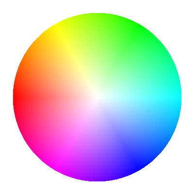
The “HSV wheel” of colors. Saturation increases from the center to the edge of the wheel.
The saturation is, therefore, a measure of the “strength” of the color relative to its brightness. Decreasing the saturation of a pixel makes it look more grayish, while increasing the saturation makes it look more vivid.
The definition of the saturation is different for the HSL color model, but the spirit is the same. In the CIELab color space, the chroma is defined as \(c^*=\sqrt{a^{*2}+b^{*2}}\), and in the CIELuv color space as \(c^*=\sqrt{u^{*2}+v^{*2}}\). The saturation is \(s^*=c^*/L^*\) in the CIELuv color space, but can not be rigorously defined in the CIELab color space (because \(c^*\to 0\) when \(L^*\to 0\) in the CIELuv, but not in the CIELab color space).
Usage
Getting and setting channels
The following method of an Image object returns an arbitrary (native or composite) channel of the image as a numpy.ndarray:
|
Return the selected channel of the image. |
where channel can be:
“1”, “2”, “3” (or equivalently “R”, “G”, “B” for RGB images): The first/second/third channel (all images).
“V”: The HSV value (RGB, HSV and grayscale images).
“S”: The HSV saturation (RGB, HSV and grayscale images).
“L’”: The HSL lightness (RGB, HSL and grayscale images).
“S’”: The HSL saturation (RGB, HSL and grayscale images).
“H”: The HSV/HSL hue (RGB, HSV and HSL images).
“L”: The luma (RGB and grayscale images).
“L*”: The CIE lightness \(L^*\) (RGB, grayscale, CIELab and CIELuv images).
“c*”: The CIE chroma \(c^*\) (CIELab and CIELuv images).
“s*”: The CIE saturation \(s^*\) (CIELuv images).
“h*”: The CIE hue angle \(h^*\) (CIELab and CIELuv images).
Alternatively, the following methods of the Image class return specific channels:
|
Return the luma L of the image. |
Return the luminance Y of the image. |
|
Return the CIE lightness L* of the image. |
|
|
Return the HSV/HSL hue of the image. |
Return the HSV value V = max(RGB) of the image. |
|
Return the HSV saturation S = 1-min(RGB)/max(RGB) of the image. |
|
Return the HSL lightness L' = (max(RGB)+min(RGB))/2 of the image. |
|
Return the HSL saturation S' = (max(RGB)-min(RGB))/(1-abs(max(RGB)+min(RGB)-1)) of the image. |
|
|
Return the hue angle h* of a CIELab or CIELuv image. |
Return the CIE chroma c* of a CIELab or CIELuv image. |
|
Return the CIE saturation s* of a CIELuv image. |
Moreover, the following functions of eQuimageLab return the luma and lightness of a numpy.ndarray (or of an Image object) containing a RGB image:
|
Return the luma L of the input RGB image. |
|
Return the CIE lightness L* of the input linear RGB image. |
|
Return the CIE lightness L* of the input sRGB image. |
A native or composite channel of an Image object can be updated with the method:
|
Update the selected channel of the image. |
Finally, a given transformation can be applied to specific channels of the image with the method:
|
Apply the operation f(channel) to selected channels of the image. |
The last two methods enable, therefore, transformations on composite channels without explicit conversions to other color spaces and models (which are handled internally by eQuimageLab). Moreover, many transformations implemented in eQuimageLab feature a channels kwarg that specifies the channels they must be applied to (see Examples below).
Histograms and statistics
The histograms and statistics of all channels can be computed with the following methods of the Image class:
|
Compute histograms of selected channels of the image. |
|
Compute statistics of selected channels of the image. |
The histograms can be displayed in JupyterLab cells or on the dashboard with the relevant commands (see First steps with eQuimageLab and The dashboard).
Also see the following functions of eQuimageLab about histograms:
Set the maximum number of bins in the histograms. |
|
Set the default number of bins in the histograms. |
Operations on the luma
Operations on the luma L of an image are designed to preserve the ratios between the RGB components, hence to preserve the HSV hue and saturation (the “apparent” color).
Therefore, stretching the luma protects the colors of the image, whereas stretching the RGB components separately usually tends to “bleach” the image. Stretching the HSV value also protects the colors, but tends to mess up the lightness (see The Image class section).
However, acting on the luma L can bring some RGB components out of the [0, 1] range.
Let us take the midtone transformation T(x) = 0.761x/(0.522x+0.239) as an example (see the Image.midtone_stretch() method). The transformation T(x) maps [0, 1] onto [0, 1] and does not, therefore, produce out-of-range pixels when applied to the R, G, B channels separately.
Let us now consider a pixel with components (R = 0.4, G = 0.2, B = 0.6) and luma L = 0.2126R+0.7152G+0.0722B = 0.271. Under transformation T, the luma of this pixel doubles and becomes L’ = T(L) = 0.543. Accordingly, the new RGB components of the pixel are (R’ = 0.8, G’ = 0.4, B’ = 1.2). While L’ is still within bounds, B’ is not.
Such out-of-range pixels are clipped when displayed or saved in png and tiff files.
There are four options to deal with the out-of-range pixels:
Leave “as is”: If you are confident that further processing will bring back these pixels in the [0, 1] range (or are satisfied with the look of the image), you can simply… do nothing about them.
Desaturate at constant luma: decrease the HSV saturation of the out-of-range pixels while keeping the luma constant until all components fall back in the [0, 1] range. This preserves the intent of the stretch (the luma is unchanged, as well as the hue) but tends to bleach the out-of-range pixels. In the present case, the transformed pixel becomes (R’ = 0.722, G’ = 0.443, B’ = 1) and the HSV saturation decreases from S = 0.667 to S’ = 0.557.
Blend each out-of-range pixel with (T(R), T(G), T(B)), so that all components fall back in the [0, 1] range. This preserves neither the luma nor the hue & saturation, and also tends to bleach the out-of-range pixels. In the present case, (T(R), T(G), T(B)) = (0.680, 0.443, 0.827) and the transformed pixel becomes (R’ = 0.736, G’ = 0.423, B’ = 1). The output luma is L’ = 0.531 and the output HSV saturation is S’ = 0.577.
Normalize the image so that all pixels fall back in the [0, 1] range (namely, divide the image by the maximum RGB value). This preserves the HSV hue and saturation, but darkens the whole image.
In eQuimageLab, these four options correspond to different choices for the kwarg channels of the midtone transformation: 1) channels = "L", 2) channels = "Ls", 3) channels = "Lb", and 4) channels = "Ln".
Alternatively, you can desaturate any overflowed Image object at constant luma with the protect_highlights_saturation() method.
Examples
The following example stretches the luma of the sRGB image image while protecting highlights by desaturation:
stretched = image.midtone_stretch(channels = "Ls", midtone = .2)
The following example increases the HSV saturation of the sRGB image image by 50% while preserving its lightness:
S = image.HSV_saturation() # Get the HSV saturation (or equivalently S = image.get_channel("S")).
S *= 1.5 # Increase the saturation by 50%.
saturated = image.set_channel("S", S) # Create a new, saturated image.
saturated.set_channel("L*", image.lightness(), inplace = True) # Correct the lightness.
Also see Image.HSX_color_saturation() for a simpler implementation of this transformation.